Portfolio of Adam Badke
A Survey of Current Techniques for Image Shadow Removal (2019)
The content below is adapted from my paper “A Survey of Current Techniques for Image Shadow Removal” submitted as a term project for SFU’s “Illumination in Images and Video” course, where I reported on my findings after implementing several techniques for the identification and elimination of shadows from digital images.
Techniques for image-based sensor sharpening, identification of an intrinsic projection direction using entropy minimization, recovering a 2D chromaticity image, and recovery of a shadow-free image with enforced re-integrability were implemented in Matlab for examination.
Beware: This is a rather long and math-heavy presentation compared to my other portfolio content! I have included it here as I personally found this course incredibly interesting, and the work is relevant to my interests in computer graphics research and development roles. Image results are included towards the end.
Abstract
There is a long history of Computer Vision research building towards the goal of removing shadows from digital images. Changes in a surface’s reflectance due to lighting, such the difference between visibly shadowed and non-shadowed regions, are visual artifacts that often prove to be challenging barriers to the success of computer vision algorithms. For example, computer vision systems can be confounded by shadows when attempting to perform segmentation, object tracking or depth reconstruction tasks.
Current, state-of-the-art methods remove shadows from digital images by clever algebraic manipulation of the properties of the computer vision model for image formation. This task is aided by retroactively performing camera sensor sharpening on image data. Chromaticity images invariant to shading changes are formed, and changes to surface reflectances due to differing lighting conditions seen as linear translations in log-chromaticity space are removed via projection onto an perpendicular intrinsic projection axis, found by evaluating entropy in the image with no knowledge of the original camera or sensors.
By comparing edges found in an image with those found in a lighting invariant version, a mask of isolated shadow edges can be obtained, and shadows can be removed by reintegrating a shadow-free version of the original image from modified gradients under conditions of enforced integrability. To demonstrate and evaluate these strategies, they are implemented and surveyed for efficacy.
1. Introduction
This paper is a survey of several published techniques for the identification and elimination of shadows from digital images. It evaluates a method for image-based sensor sharpening [1], combined with a technique for recovering lighting-invariant 2D chromaticity images using entropy minimization [2, 3, 4], which are used to obtain a mask of isolated shadow edges. Finally, the use of shadow edge maps for removing shadow edge gradients is evaluated; modified image gradients are reintegrated with a method for enforcing integrability [5] to recover shadow-free versions of the original RGB images.
The goal of this paper is to evaluate the efficacy of each of these techniques in isolation from, and in combination with, each other. To this end, the implementation in this paper is compared against the best-case results published in prior works, and those obtained using hand-created masks. Visual comparisons of the output throughout the shadow removal process are provided to illustrate the steps most influential towards achieving high-quality results with these techniques.
2. System Model
2.1 Model of Image Formation
This paper uses the standard computer vision model for 3-channel RGB image formation. For a pixel value \(R_k(x,y)\), \(k = 1…3\), we have:
\(R_k(x,y)=w(x,y)\int E(x,y,\lambda_k)S(x,y,\lambda_k)Q_k(\lambda)d\lambda\)
Here, for each \(pixel(x,y)\) in an image, \(w(x,y)\) denotes the shading term of the surface at the sampled location. The total aggregated contribution of illumination at \(pixel(x,y)\) is the integral over the light spectra reflected to the camera sensor for each RGB channel. \(E(x,y, \lambda_k)\) denotes the incoming spectral power distribution illuminating the surface, and the surface reflectance is described by \(S(x, y, \lambda_k)\). Finally, \(Q_k(\lambda)\) describes the camera sensitivity functions for each of the 3 image channels.
Following the examples set in prior works [2,3], we make several assumptions for this model: We assume a Lambertian shading term for \(w(x,y)\), and for \(S(x,y,\lambda_k)\), we assume narrow-band camera sensor response curves described by a Dirac delta function:
\(Q_k(\lambda) = q_k\delta(\lambda-\lambda_k)\)
Finally, we use Wein’s approximation of Planck’s lighting model:
\(E(\lambda, T) \simeq Ik_1\lambda^{-5}e^{\frac{-k_2}{T\lambda}}\)
2.2 Finding an Intrinsic Image
Again, we follow the examples set by prior works [2,3] towards the goal of finding a lighting-invariant image by forming band-ratio log chromaticities from source RGB images. First, the incoming RGB image is pre-filtered before processing: It is linearized to remove gamma correction, and then a Gaussian blur is applied to remove high-frequency noise from the image.
Next, for each \(pixel(x,y)\) in our filtered RGB image, we compute the geometric mean:
\(\mu = \sqrt[3]{R\cdot G\cdot B} \)
The geometric mean is used as the denominator when forming band-ratio chromaticities for each RGB channel, as it avoids biasing one particular channel when computing our lighting-invariant image, while maintaining the desirable properties of linear changes under varied lighting temperatures, \(T\), observed in log-chromaticity space.
Band ratio log chromaticities are formed as follows:
\(\chi_k(x,y) = log(R_k(x,y)) – log(\mu(x,y) = log(\frac{R_k(x,y)}{\mu(x,y)}) \)
The division operation (i.e. log-space subtraction) cancels the shading term \(w(x,y)\) and lighting intensity term \(I\) described at our pixel above. Thus, we’re left with a relationship describing our RGB surface reflectances independent of shading or intensity, dependent only a translation of \(T\) in log space. As shown in prior works [4], when a surface is measured under different illumination conditions, illumination changes in log space are described by a linear translation; plots of pixel values for surfaces captured under differing illumination conditions lie on approximately parallel lines.
2.3 Projecting from Log Chromaticity to 2D Plane Space
2.4 Entropy Minimization
To locate the ideal invariant projection direction, we use the entropy minimization technique described in [2]. In this context, entropy describes the clustering of log chromaticity band ratio values on a candidate invariant projection axis after projection has been performed. A projection is said to have low entropy when pixels describing similar surface reflectances are tightly clustered together after the projection. A projection is said to have high entropy when the projection results in even, or seemingly random distributions of values along the projection axis.
To identify the ideal invariant projection angle we perform a brute-force search, forming candidate projection directions for each angle between 0° and 180°. Each angle is tested for suitability by projecting the image’s log chromaticity band ratios onto it, and evaluating the resulting entropy. The angle resulting in the lowest entropy is chosen as the ideal invariant projection angle.
The entropy of a projection is computed by forming a histogram of equally-spaced bins containing the resulting projected values. Only the middle 90% of values are considered; the top and bottom 5% of values are considered as outliers and discarded. For the bins that are occupied, we divide by the sum of the total bin counts to find probability \(p_i\). The final entropy value of a projection is computed as:
\(\sum_{i=1}^{n} –p_i \cdot log_2(p_i)\)
2.5 Improving the Chromaticity Image
As described in prior works [3], a 2D-color invariant image better-behaved than a greyscale invariant image can be found by remapping the log chromaticity lighting information using the brightness of the top quartile of the original image’s brightest pixels. A regression is performed to find the optimal \(3\times3\) transformation matrix adhering to the following constraints:
\(min\sum (\rho_{orig}, brightest quartile – M\hat{\rho} )^2\)
\(\sum M_i = 1, i = 1…3\)
\(0 \leq M \leq 1\)
Where \(\rho\) is our original image, \(\hat{\rho}\) is our log chromaticity image, and \(M\) is the target transformation matrix. Transforming the chromaticity with \(M\) consistently re-illuminates the image without regard to the differences between in/out of shadow regions.
2.6 Image-Based Sensor Sharpening
The computer vision image formation model used here assumes narrow-band camera sensor response curves with Dirac delta functions. In practice, this is inaccurate for RGB images captured from a typical camera. Thus, to optimize the results of our entropy minimization process, we use the technique described by [1] to find a sensor sharpening transformation matrix through a minimization optimization applied to our incoming RGB image before the entropy minimization process is performed.
Here, the sensors are retroactively sharpened to be narrower band by transforming the image data with no knowledge of the camera sensors. Pixels identified by a user-supplied binary mask indicating regions both in and out of shadow are concatenated into a single array, which is then used to drive an optimization solver for a \(3\times3\) sharpening matrix \(M\).
The ideal \(M\) is one that results in the lowest overall entropy for the selected pixels after the transform is applied. As per [1], the minimization optimization is constrained as follows:
\(\overset{\mathrm{min}}{M} f(M, P) = \alpha \times rank(M)\)
Where:
\(\sum_{j=1}^{3} M_{ij} = 1, i = 1…3\)
\(|M_{ii} – 1| \leq \beta\)
\(M_{ij}| \leq \beta\)
Matrix \(M\) is desired sharpening matrix, and \(P\) is the concatenation of the pixels indicated by the user-defined mask. The constant \(\alpha\) controls the rank constraint (As per [1], alpha = 0.05 is used), and \(\beta\) constrains the changes in the sensor to maintain the primary color hue (Again, as per [1], \(\beta\) = 0.3 is used). \(\chi\) represents our log chromaticity band ratios, and \(\theta\) is our candidate invariant projection angle. Finally, a non-integer rank function is defined as:
\(rank = \frac{\lambda_3}{\lambda_1}\)
Where \(\lambda_i, i = 1…3\) are the singular values from the SVD decomposition of \(M\). When solving the optimization problem, we test each candidate sharpening matrix \(M\) against possible projection angles from 0° to 180°, to locate the transformation that results in the lowest overall entropy.
2.7 Finding Shadow Edges
Now that we sharpened our input image and found the projection angle resulting in the lowest entropy after projection, we’re able to compute a best-case lighting invariant image. In this image, shadows and lighting information have been removed, yet edge structure is otherwise relatively unchanged. That is to say, when evaluating the edges in our incoming and intrinsic images, the primary difference is that the intrinsic image lacks shadow edges.
As in [2], we capitalize on this difference to construct an edge mask containing shadow edges alone. This is achieved by running Canny edge detection on both the incoming image, and the intrinsic image to achieve 2 binary edge masks: \(\nabla I_{orig}\), consisting of edges in the original image, and \(\nabla I_{inv}\), consisting of edges in the invariant image. Then, shadow edges \(\nabla S\) can be isolated using the following logical AND operation:
\(\nabla S = \nabla I_{orig} \& \neg \nabla I_{inv}\)
Where \(\neg \nabla I_{inv}\) is the logical NOT of the binary edge mask found for the invariant image.
2.8 Recovering a Shadow-Free Image
In this final step, the shadow edge mask is used in combination with the enforced integrability technique described in [5] to recover a shadow-free version of the input image. First, the per-channel gradient of the original image is found by convolving each channel in both the x and y directions with a simple gradient kernel, \([-1, 1]\). Then, using the (morphologically inflated) shadow edge mask, derivatives describing shadows edges are set to 0.
Reintegration from the modified gradient image to a shadow free version of the original color image is performed, per-channel, in the Fourier domain. First, the boundaries of the image are wrapped around to form the periodic image expected by the Fourier transform. Then, we transform the derivatives into Fourier space, and reintegrate the original image from our modified derivatives by projecting onto an integrable basis as described in [5]. Upon returning from Fourier space, the shadows have been removed from our image.
3. Results
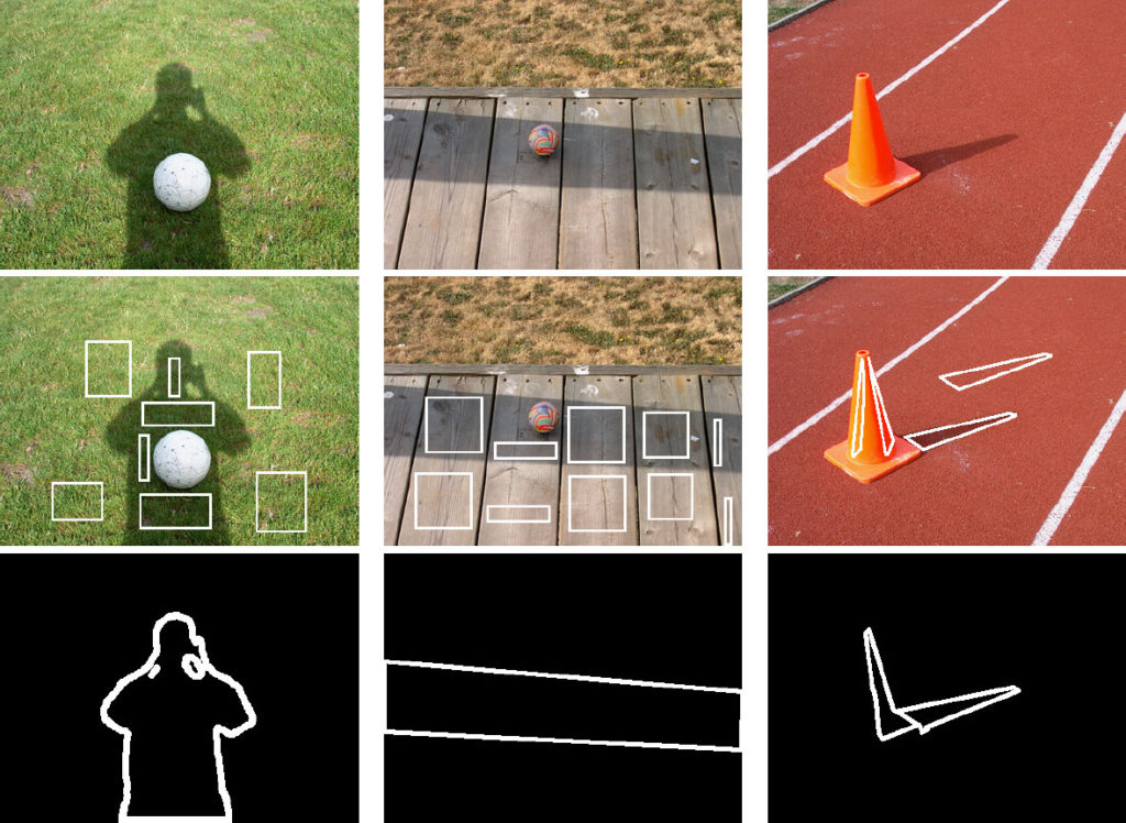
3.1 Input Images and User-Defined Masks
Source images with known results from previous works [2] were used to evaluate the techniques described above. 3 RGB images were selected for their diversity in dominant color and texture, and hand-created selection masks for regions of pixels in/out of shadows (pictured below as borders surrounding the selected regions), and “perfect” hand-drawn edge maps were created.
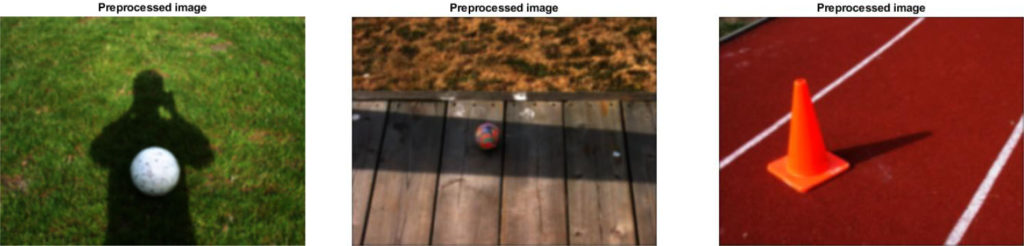
3.2 Image Pre-processing
The input images were pre-processed before the shadow removal process began. Each image was linearized to remove gamma correction, then a Gaussian blur applied to remove high frequency noise, and finally, 0’s in the image channels are replaced by 1/255.
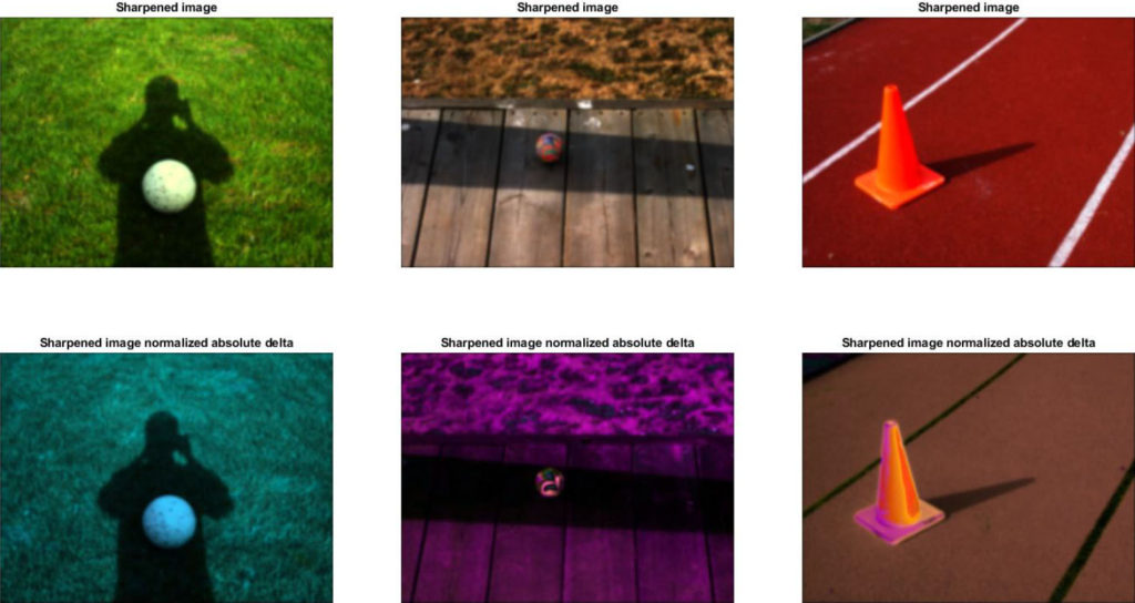
3.3 Sensor Sharpening Results
The results of performing image-based sensor sharpening on the input images are shown below. A normalized, absolute value result of the difference between the pre-processed image and the sharpened image are included, revealing the dominant color shift resulting from the sharpening transformation. The following sharpening matrices were found for each respective image (Note: The matrices are row-major, where each row represents the transformation weighting for a single RGB channel):
\(
\begin{bmatrix}
1.0041 & 0.1442 & -0.1483 \\
-0.0412 & 1.0990 & -0.0578 \\
0.0823 & -0.0702 & 0.9878 \\
\end{bmatrix}
\)
\(
\begin{bmatrix}
1.0000 & 0.0000 & 0.0000 \\
0.0000 & 1.0000 & 0.0000\\
0.0000 & 0.0000 & 1.0000\\
\end{bmatrix}
\)
\(
\begin{bmatrix}
1.0511 & -0.0323 & -0.0188 \\
-0.0323 & 1.0644 & -0.0321 \\
-0.0188 & -0.0321 & 1.0509 \\
\end{bmatrix}
\)
From top to bottom: Sensor-sharpening matrices for ball on grass, ball on wooden path, and cone images
Compared with the noticeably color-shifted results demonstrated in [1], the effect of sensor sharpening here appears mild. The sharpening matrix found for the image of the ball on the wooden path was the identity matrix, leaving the image unchanged. The ball on the grass, and the cone images were modified, but the change is barely perceptible. Inspecting the rows of their sharpening matrices provides a clue as to why: While a weighting change of up to 30\% was permitted by the sharpening optimization constraints, the maximum change for a channel value was less than \(\approx15\%\) of the previous values. It is likely that the lack of diversity in pixel colors for the selected in/out of shadow regions, particularly for the image of the ball on the wooden path, made it difficult for the minimization optimization to converge on a meaningful result.
Perhaps supplying the program with masks selecting different pixels, or modifying the constraints of the minimization optimization routine would provide more noticeable results. However, this algorithm is not intended to be tuned for the visual sensitivities of human sight; it’s possible that these transformations are indeed ideal (although this is unlikely, given the poor results for the image of the ball on the wooden path throughout this paper in general). Comparison of the influence of sensor sharpening on the intrinsic projection direction found against the ideal calibrated result is a more meaningful benchmark (See section 3.5).
3.4 Log Chromaticity Band Ratios
Plots of the log chromaticity band ratios projected to 2D plane space are provided to allow comparison between the projected data with and without sensor sharpening. As the sharpening matrix found for the image of the ball on the wooden path was the identity, there is no change to the projected data. However, for the remaining 2 images (the ball on the grass, and the cone), the changes due to spectral sharpening are evident. Both plots show points more closely clustered together after spectral sharpening has been applied.
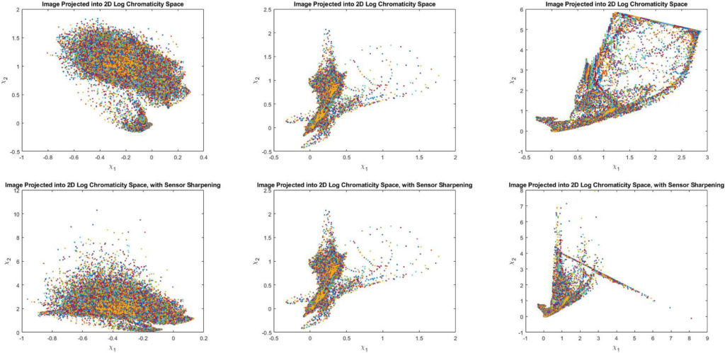
From top to bottom: Projections with no prior sensor sharpening, projections after sensor sharpening. From left to right: Image of a ball on grass, image of a ball on a wooden path, image of a cone on a running track
3.5 Entropy Plots
Both with and without sensor sharpening applied, the general shape of the entropy curves for all 3 images appear relatively similar. Again, we see only minor changes due to sensor sharpening. The best intrinsic projection angle found using the entropy minimization technique was influenced differently for each of the test images. Unsurprisingly, the angle found for the image of the ball on the wooden path was not affected at all; using the identity matrix as a sensor sharpening transformation did not alter the outcome of the entropy minimization procedure.
For the image of the ball on grass, sensor sharpening resulted in a smoother curve and a 7° change in the identified projection angle. Interestingly, the instrinsic projection angle found was \(\approx\)70° away from the results reported in [2], but the final shadow removal result achieved with this angle is impressive. For the image of the cone, while sensor sharpening has visibly sharpened the plotted curve, the identified best projection angle is unchanged.
Interestingly, the projection angles found using entropy minimization for the images of the ball on grass, and the ball on the wooden path, are significantly different to those demonstrated in [2], both with and without sensor sharpening. Yet, the image of the cone on the track is only 2° from the results of [2]. These results are inconsistent with the previously published work, pointing to a potential issue with the implementation of the described algorithms, although after careful comparison of the code against the procedures described in the source material no obvious issues could be found.
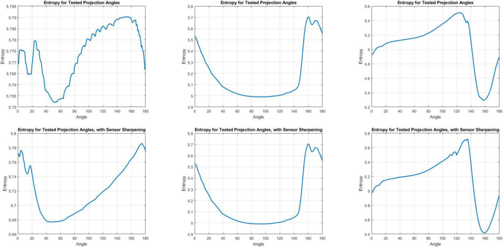
From top to bottom: Entropy results with no spectral sharpening, entropy results after spectral sharpening
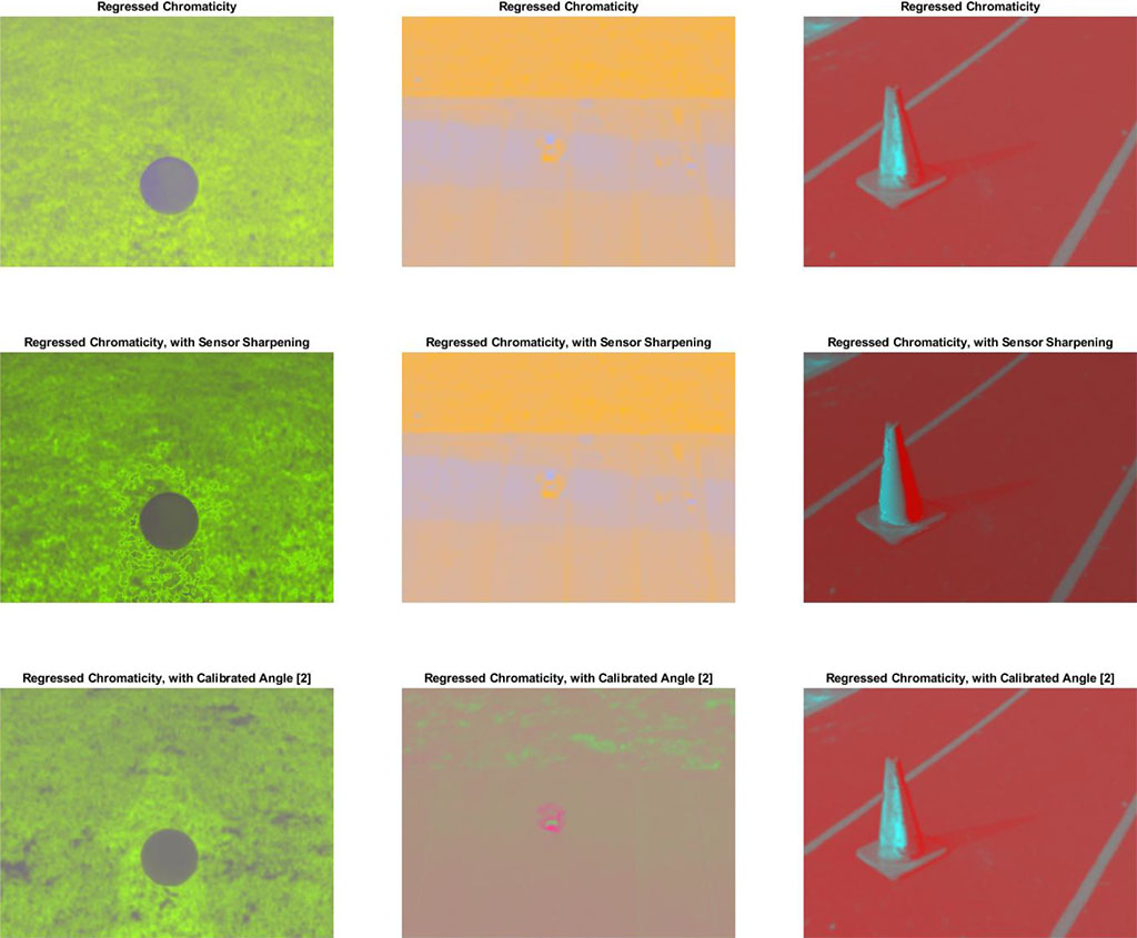
3.6 Re-Illuminated Chromaticity Results
Here, the results of re-illumination of chromaticity images using the median brightness of the top 1% of each image are shown for visual comparison. In addition to the chromaticity images found with/without sensor sharpening, the resulting chromaticity image computed using the intrinsic projection angle found for a HP912 camera via calibration in [2] is also shown. Visual inspection reveals mixed results for each of the test images.
For the image of the ball on grass, the chromaticity image found without sensor sharpening has the least noticeable shadow artifacts remaining after regression. Interestingly, the worst result seems to occur when using the intrinsic projection angle found by calibration in [2].
The image of the ball on the wooden path had very poor results; shadows can still be clearly seen in the chromaticity images found using entropy minimization both with and without sensor sharpening. However, the shadows appear to be completely removed in the chromaticity image derived by using the intrinsic projection angle derived by calibration in [2], again suggesting the source image or the entropy minimization technique implemented for this paper somehow differ from the original work.
Finally, the image of the cone appears remarkably similar after regression in all 3 images.
It is worth noting that subjective evaluation of the chromaticity images should be taken with a grain of salt; human visual perception is flawed when performing subjective evaluations of similar colors and shades. The true value of these images lays in the quality of the edge maps that can be recovered from them.
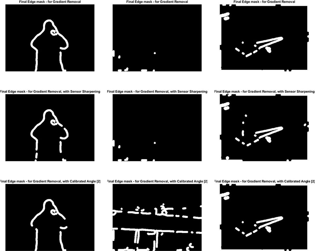
3.7 Shadow Edge Masks
The final quality of the recovered, shadow-free image is almost entirely dependent on the quality of the shadow edge mask. Computing a mask that accurately represents the true and complete shadow edges in the original image, while minimizing the number of erroneous edges in the final result, is the goal of all of the work performed so far.
To enable consistent output comparisons, a single set of tuning parameters was chosen for each image that resulted in the cleanest output edges that could be obtained from the intrinsic image found using the “best case” calibrated intrinsic projection angle identified in [2]. To enable fair comparisons between the sets of edges obtained from the various versions of each image’s intrinsic images, the same tuning parameters were used for all edge detection passes of an image’s intrinsic versions. The decision to tune edge detection for the intrinsic image obtained using the calibrated intrinsic projection angle was made on the assumption that the calibrated result would be superior; however the results, particularly for the image of the ball on the wooden path, show this assumption was not always correct.
For the image of the ball on grass, the edges found by by entropy minimization alone, without employing sensor sharpening are the most accurate, connected, and noise-free in comparison with the known position of the shadow edges in the original image. Similarly, for the image of the cone, the edges found by entropy minimization alone are visually indistinguishable from the edges obtained using the ideal projection angle identified in [2]. Surprisingly, in both cases, spectral sharpening resulted in slightly lower quality edges, with more discontinuities and noise.
For the image of the ball on the wooden path, finding an edge mask using entropy minimization, both with and without sensor sharpening, was a complete failure. This is likely due to the significant differences in the regressed chromaticity images found prior; the Canny edge detection routine was tuned for best performance with the visibly different intrinsic image found using the calibrated projection angle for the HP912 camera found in [2]. However, despite this, even these best-case edges are noisy and disconnected. It is highly probably that tuning the edge detection differently for this image would improve the results.
3.8 Reintegration with Shadows Removed
Now that shadow edge masks have been computed, it’s possible to recover and evaluate the final, shadow-free versions of the input images. In addition to results found with computed shadow edge maps, results found using hand-painted shadow edge maps are also provided for best-case comparison. Encouragingly, for all of the test images, high-quality, shadow-free output was obtained in several, and in some cases all, of the test cases.
In the image of the ball on grass, the results using entropy minimization with and without sensor sharpening, as well as when using the calibrated intrinsic projection direction, are of similarly high-quality. While not removed completely, the visibility of the shadow has been significantly reduced. The best-case output obtained using hand-painted edge maps is visually superior; this is likely due to the shadow edge painted on the bottom edge of the image that is not present in the computed shadow maps. Future work into detecting shadow edges at image borders would likely result in the quality of the automated results approaching that of the best-case for this image.
For the image of the cone, the results obtained using entropy minimization with and without sensor sharpening, as well as when using the calibrated intrinsic projection direction, are arguably approaching the same quality level as the best-case output found with a hand-painted edge map. Of note, the image obtained with hand-painted edges has the shading removed from the back side of the cone, which is still visible in the images obtained with computed edge maps. The hard shadow of the cone cast onto the track is almost completely removed from all images. While some artifacts caused by the small amounts of noise in the computed edge maps are still visible in the final image, the results are of equivalently high quality for the most part. This image does not suffer the darkening effect caused by missing shadow edges along the image boundaries as seen in the other images.
Unsurprisingly, for the image of the ball on the wooden path, the shadows remain entirely visible after using entropy minimization, both with and without sensor sharpening, due to the poor quality of the obtained shadow edge maps. However, when edges found in the intrinsic image computed with the calibrated intrinsic projection direction from [2] are used, the results are very high-quality, with the shadows almost completely removed. Similar to the image of the ball on grass, again we see an improvement when using hand-painted shadow edge maps due to the edges painted where the shadows intersect with the image edge.
These results are highly encouraging; a shadow-free image could be recovered with only minor artifacts for each of the test images. The quality of these images confirm that entropy minimization is a viable strategy for shadow removal. Additionally, the high-quality results obtained using hand-painted shadow edge maps highlight the importance of obtaining accurate shadow edge locations to remove shadow edge gradients before reintegration.
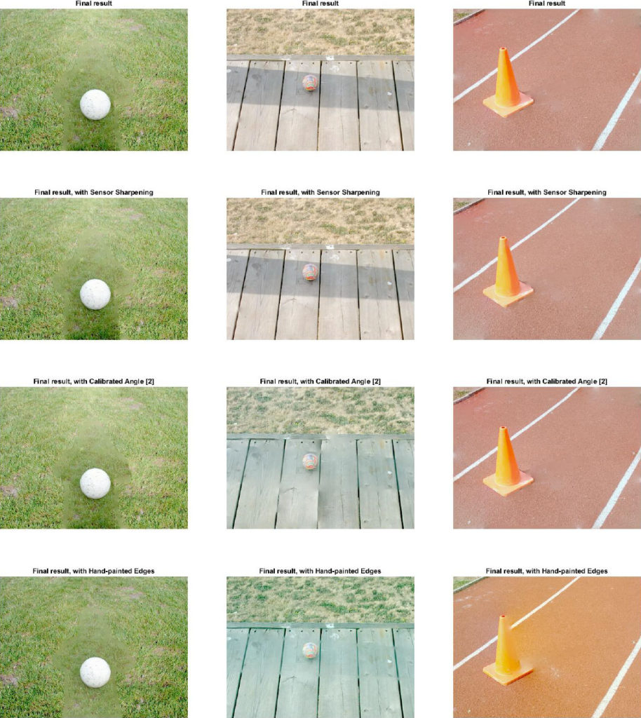
From top to bottom: Result using entropy minimization, result using sensor sharpening and entropy minimization, result using calibrated invariant projection direction from [2], result using a hand-painted edge mask.
4. Summary and Conclusions
This survey of current shadow removal techniques confirms the methods and findings described in the source material [1,2,3,4,5] are indeed valid. While the results found with sensor sharpening were underwhelming, this technique should not be discredited as further investigation into tuning and optimization may yield more significant results. Despite this, the entropy minimization technique proved itself a promising replacement for device-specific calibration in producing light-invariant 2D chromaticity images with heavily reduced or even completely eliminated shadow visibility. Finally, assuming a high-quality shadow edge mask can be found, this paper confirms it is possible to reintegrate a shadow-free version of an image from modified gradients with only minor artifacts.
Future work towards improving the results explored in this paper should focus in 2 main areas: Improving the results of the entropy minimization technique to find an intrinsic projection direction closer to what would be found through calibration, and finding higher quality edge maps without the need for per-image tuning parameters. It is possible (and probable) that the differences between the implementation used to perform this survey and the published works being evaluated [1,2,3,4,5] was lacking insights known to the original authors, influencing the results obtained. However, the results demonstrated here highlight how if an ideal intrinsic projection direction is found, a lighting invariant chromaticity image can be computed, allowing high-quality shadow edge maps to be isolated, and a high-quality shadow-free version of the original image with minimal artifacts can be recovered.
All of the techniques surveyed in this paper – image-based sensor sharpening, identification of an intrinsic projection direction using entropy minimization, recovering a 2D chromaticity image, and recovery of a shadow-free image with enforced re-integrability – show great promise and warrant further investigation, exploration, and improvement.
Acknowledgments
This work is based on the work of Dr. Mark Drew of Simon Fraser University, with permission.
References
- M. S. Drew and H. R. V. Joze, “Sharpening from Shadows: Sensor Transforms for Removing Shadows using a Single Image,” Courtesy of Simon Fraser University
- G. D. Finlayson, M. S. Drew, and C. Lu, “Intrinsic Images by Entropy Minimization,” ECCV 2004, pp. 582–595, 2004.
- M. S. Drew, G. D. Finlayson, and S. D. Hordley, “Recovery of Chromaticity Image Free from Shadows via Illumination Invariance,” ICCV’03 Workshop on Color and Photometric Methods in Computer Vision, Nice, France, pp. 32–39.
- G. D. Finlayson and S. D. Hordley, “Color Constancy at a pixel,” Optical Society of America, Aug. 2000.
- R. T. Frankot and R. Chellappa, “A Method for Enforcing Integrability in Shape from Shading Algorithms,” IEEE Transactions on Pattern Analysis and Machine Intelligence, vol. 10, no. 4, pp. 439–451, Jul. 1988.